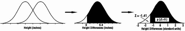
The effect size (d) is equivalent to a 'Z-score' of a standard normal distribution.
The Common Language Effect Size (CLE) is closely related to Pr (Z> x) and is used to interpret an effect size by converting an effect into a probability.
Hattie borrowed the CLE from McGaw and Wong (1992, p. 361) which they defined as,
"the probability that a score sampled at random from one distribution will be greater than a score sampled from some other distribution."
Hattie used the example from McGaw and Wong (1992) of the differences in height between men and women (p. 362). If a man and women are sampled randomly, the chance the man will be taller than the women is pr (z > -1.41) or around 92% as shown below:
However, Hattie has calculated CLE probability values of between -49% and 219%. The researchers, Higgins and Simpson (2011), Topphol (2011) and Bergeron & Rivard (2017) identified that these values are not possible.
Bergeron & Rivard (2017) state,
Professor Arne Kare Topphol, who published that Hattie had calculated CLE's incorrectly in his paper, 'Can we count on the statistics use in education research?' had a dialogue with Hattie:

However, the table heads 12 Meta-analyses, but there are clearly 13 meta-analyses & this error prompted me to check the average.
This is important as this particular result contradicts one of Hattie's fundamental claims,
Hattie mixes up the X\Y Axis:
Hattie uses a funnel plot (p. 21) to show that publication bias does not affect his research. But, Higgins and Simpson (2011) show that Hattie has mixed the X/Y axis and if drawn correctly the funnel plot does, in fact, show publication bias (p. 198).
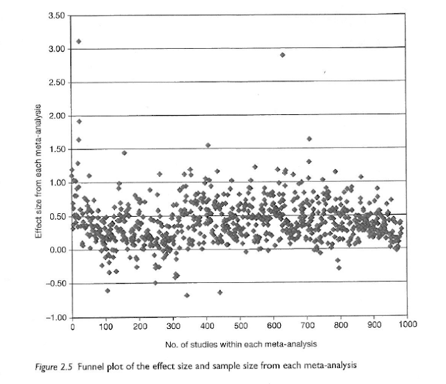
Yelle et al. (2016) 'What is visible from learning by problematization: a critical reading of John Hattie's work', say there is an implied underestimation of the publication bias in Hattie's synthesis.
This is a significant study as it attempts to deal with many of issues & mistakes of Visible Learning that have been raised in the peer review (and often denied by Hattie - see Hattie's Defenses).
In regards to publication bias they reject 8 of the original 23 feedback studies that Hattie used in VL & significantly reduce the impact of a further 11/23 of those studies.
There are many examples of this error, e.g., Hattie (VL, p. 87) cites Dustmann et al., (2003) with effect size -0.04. But, Dustmann et al., found that the larger the class, the worse the test performance, i.e., the paper's reference point is INCREASING class size NOT reducing class size (which is Hattie's reference point) so the effect size should be +0.04.
However, Hattie has calculated CLE probability values of between -49% and 219%. The researchers, Higgins and Simpson (2011), Topphol (2011) and Bergeron & Rivard (2017) identified that these values are not possible.
Bergeron & Rivard (2017) state,
"To not notice the presence of negative probabilities is an enormous blunder to anyone who has taken at least one statistics course in their lives. Yet, this oversight is but the symptom of a total lack of scientific rigor, and the lesser of reasoning errors in Visible Learning."
Topphol (2011) states,
"I will show that Hattie makes a systematic mistake in his calculations of CLE. In addition, his judgement, on how a calculated CLE should be interpreted in the context, suggests that he misunderstands what information CLE provides." (p. 463, Translated).
As a result, Hattie finally has now admitted that he calculated all CLE incorrectly. Although, he now says the calculation was not important. However, originally he did say that,
"in all examples in this book, the CLE is provided to assist in the interpretation of the effect size" (p. 9).
Given Hattie's mantra that interpretations are the important aspect of his synthesis, this is a significant mistake.
Topphol (2011), details that Hattie's explanations of particular CLE's are also incorrect, e.g., an effect size d = 0.29 must create a CLE of at least 50%. Excerpt from VL p. 9,

Topphol (2011) shows this interpretation is not correct on a number of levels,
Topphol (2011) shows this interpretation is not correct on a number of levels,
"On page 9 Hattie give an example to help the reader interpret the CLE. “Now, using the example above, consider the d = 0.29 from introducing homework […]. The CLE is 21 per cent […]” First, 21 per cent is not correct, it should be approximately 58 per cent. The example continues “[…] so that in 21 times out of 100, introducing homework into schools will make a positive difference, or 21 per cent of students will gain in achievement compared to those not having homework”. This interpretation is not correct, and it would not have been even with the correct percentage.
The CLE does not tell us how many students that gain in achievement, with a CLE of 58 per cent it is in fact possible that every student gain in achievement. In this context a correct interpretation would be that a CLE of 21 per cent (58 per cent) means that if you draw a random pair of students, one from the population with homework and the other from the population without (otherwise identical populations), there would be a probability of 21 per cent (58 per cent) that the student with homework achieves higher than the one without. This is not equivalent with Hattie’s explanation."
Ecological Fallacy, Topphol again,
'Hattie continues his explanation: “Or, if you take two classes, the one using homework will be more effective 21 out of a 100 times”. His interpretation of the percentages is now correct, but he seems to make what is often referred to as an ecological fallacy.'
It is not obvious what he means by one class is more effective than the other class. Nevertheless, what he writes indicates strongly that he means that an effect size, here a CLE, on an individual level can be transferred unchanged to the class level. First he writes about an effect on student level, the on the class level, using the same effect size value. This is not correct. The effect size on class level will, in normal circumstances, be larger than on student level, often noticeable larger.'
Topphol provides the following simulation,
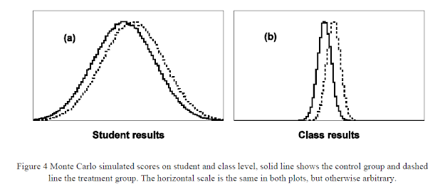
"A computer program has been used to draw random samples of student scores from given population distributions using a Monte Carlo method (see e.g. Mooney 1997 or Rubinstein & Kroese 2008). In figure (a) the results for one million individual students are shown. Half of the students were randomly chosen to constitute a control group and the rest went into a treatment group. The two curves, solid and dashed, show how the students’ results were distributed. The difference between the two distributions corresponds to an effect size d = 0.30 .
The students were then randomly grouped together in classes of 20 students each. For every class a class score were calculated as the arithmetic mean of the individual student scores. The class score distributions are plotted in figure (b), both control and treatment classes. The difference between the mean values is the same in (a) and (b), but the standard deviations are substantially reduced in (b), as expected from the central limit theory. Calculating the class effect size gives d = 1.34 , a factor of 4.46 larger than the individual effect size, also as expected; a substantial increase in effect size. Converted to CLE we get 58 per cent on student level and 82 per cent on class level.
...it is nevertheless a mistake to directly transfer an effect size from student to class level. When Hattie in his example uses the same value of CLE on class level as on student level, it is an ecological fallacy."
More Errors
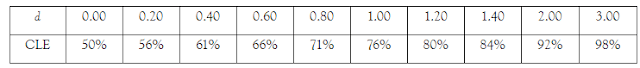
Then again on page 42, Hattie makes the same error citing d = 0.67 has a CLE of 48%. But 48% would indicate a negative d value. See table 1 from Bergeron (2017),
TABLE 1. Correspondence between Cohen’s d and CLE equivalents
TABLE 1. Correspondence between Cohen’s d and CLE equivalents

Professor Arne Kare Topphol, who published that Hattie had calculated CLE's incorrectly in his paper, 'Can we count on the statistics use in education research?' had a dialogue with Hattie:
"My criticism of the erroneous use of statistical methods will thus probably not affect Hattie’s scientific conclusions. However, my point is, it undermines the credibility of the calculations and it supports my conclusion and the appeal I give at the end of my article; when using statistics one should be accurate, honest, thorough in quality control and not go beyond one's qualifications.
My main concern in this article is thus to call for care and thoroughness when using statistics. The credibility of educational research relies heavily on the fact that we can trust its use of statistics. In my opinion, Hattie’s book is an example that shows that we unfortunately cannot always have this trust.
Hattie has now given a response to the criticism I made. What he writes in his comment makes me even more worried, rather than reassured."Topphol was referring to Hattie's response that he used a slightly different formula and that resulted in these strange values.
Hattie stated,
"Yes, I did use a slightly different notion to McGraw and Wong. I struggled with ways of presenting the effect size data and was compelled by their method – but … I read another updated article that was a transformation of their method – but see I did NOT say this in the text. So Topphol’s criticism is quite reasonable. I did not use CLE exactly as they described it!" Read full dialogue here.Hattie (2015) in a later defence of his work, contradicts the explanation he gives in 2012 to Topphol above, i.e., that he used a different calculation to Topphol:
"at the last minute in editing I substituted the wrong column of data into the CLE column and did not pick up this error; I regret this omission."
But this does not explain Hattie's incorrect use of the CLE probability statistic in VL (2009, p. 9&42) as mentioned by Topphol above.
Hattie no longer promotes the CLE as a way of understanding his effect sizes, he uses a value of d = 0.40 as being equivalent to 1 year's progress. But as already stated, this creates other more significant problems.
Another Blog which discusses these CLE issues - http://literacyinleafstrewn.blogspot.com/2012/12/can-we-trust-educational-research_20.html
The Power of Feedback - Hattie & Timperley (2007)
Hattie based Visible Learning on his 2007 article, "The Power of Feedback". Hattie & Timperley collected 13 Meta-analyses and averaged their effect sizes, table 1-

However, the table heads 12 Meta-analyses, but there are clearly 13 meta-analyses & this error prompted me to check the average.
Hattie & Timperley (2007) summarise,
"At least 12 previous meta-analyses have included specific information on feed back in classrooms (Table 1). These meta-analyses included 196 studies and 6,972 effect sizes. The average effect size was 0.79." (p. 83)
However, if you average the effect sizes from the table above you get 0.53 NOT 0.79, which totally changes Hattie's narrative about the "high" impact of feedback. Also, the effect column does not tally to anything near 6,972!
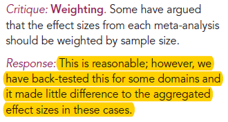
A possible reason for the different averages is weighting. But, Hattie has been heavily criticised for not weighting - see Effect Size, problem 8.
And, Hattie defended against these critiques in Hattie & Hamilton (2020),

In what Hattie says is the most systematic study on feedback, Kluger & DeNisi (1996), he cites their figure of 32% of effects of feedback decrease Achievement (Hattie & Timperley (2007), p. 85) and repeats this in Visible Learning (p. 175).
"When teachers claim that they are having a positive effect on achievement or when a policy improves achievement, this is almost always a trivial claim: Virtually everything works. One only needs a pulse and we can improve achievement." (VL p. 16).
Well clearly in his most reliable Feedback study, a significant number of feedback strategies DO NOT WORK!
It would be much more useful for teachers to know, what does not work, which is what the Kluger & DeNisi paper spends a significant time on trying to figure out.
Hattie mixes up the X\Y Axis:
Hattie uses a funnel plot (p. 21) to show that publication bias does not affect his research. But, Higgins and Simpson (2011) show that Hattie has mixed the X/Y axis and if drawn correctly the funnel plot does, in fact, show publication bias (p. 198).
Yelle et al. (2016) 'What is visible from learning by problematization: a critical reading of John Hattie's work', say there is an implied underestimation of the publication bias in Hattie's synthesis.
Kraft (2022) in his discussion with Hattie, challenges many of Hattie's contentions,
"Publication bias, where lots of studies of ineffectual programs are never written or published, further strengthens my suspicion that the 0.40 hinge point is too large."
Dr. Ben Goldacre on the Funnel Plot

For more information see - https://en.wikipedia.org/wiki/Funnel_plot
Hattie Finally Uses the Correct funnel Plot
For more information see - https://en.wikipedia.org/wiki/Funnel_plot
Hattie Finally Uses the Correct funnel Plot
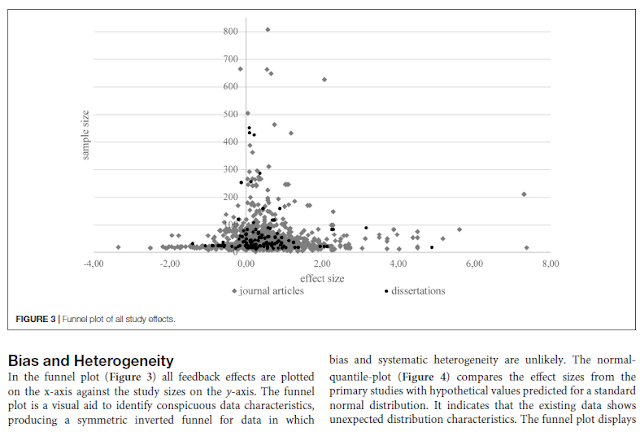
In Wisniewski, Zierer & Hattie (2020) "The Power of Feedback Revisited", there is more of an effort to deal with the publication bias issue (as well as other issues), they publish a correct funnel plot for feedback (p. 8),

This is a significant study as it attempts to deal with many of issues & mistakes of Visible Learning that have been raised in the peer review (and often denied by Hattie - see Hattie's Defenses).
In regards to publication bias they reject 8 of the original 23 feedback studies that Hattie used in VL & significantly reduce the impact of a further 11/23 of those studies.
As a result, the average effect size reduced dramatically from 0.79 in 2007, then 0.73 in VL to 0.48 in this study.
This means a complete reframing of the "story" Hattie created about feedback in classrooms. In fact, they completely contradict Hattie's original claims in VL,
"...the significant heterogeneity in the data shows that feedback cannot be understood as a single consistent form of treatment." (p. 1)
Hattie Does Not Adjust for the Reference Point of Studies & Reports -ve effect size instead of +ve effect size (or vice versa)
Professor Robert Slavin (2018) in his blog John Hattie is Wrong, also provides another pertinent example of Hattie's error,
"A meta-analysis by Rummel and Feinberg (1988), with a reported effect size of +0.60, is perhaps the most humorous inclusion in the Hattie & Timperley (2007) meta-meta-analysis. It consists entirely of brief lab studies of the degree to which being paid or otherwise reinforced for engaging in an activity that was already intrinsically motivating would reduce subjects’ later participation in that activity. Rummel & Feinberg (1988) reported a positive effect size if subjects later did less of the activity they were paid to do. The reviewers decided to code studies positively if their findings corresponded to the theory (i.e., that feedback and reinforcement reduce later participation in previously favored activities), but in fact their “positive” effect size of +0.60 indicates a negative effect of feedback on performance.
Standard ErrorI could go on (and on), but I think you get the point. Hattie’s meta-meta-analyses grab big numbers from meta-analyses of all kinds with little regard to the meaning or quality of the original studies, or of the meta-analyses."
"In his "Effect Barometers" Hattie also gives a standard error for the determined effect size. However, their calculation is flawed (see also Pant 2014 a, p. 96, note 4, 2014b, p. 143, FN 4). As a rule, the specified value is the arithmetic mean of the specified standard errors of the individual first-stage meta-analyzes. For example, in the case of inquiry-based teaching, the given standard error of 0.092 is the arithmetic mean of the two standard errors of 0.154 and 0.030 given two of the four meta-analyzes. However, the precision of the estimate from both meta-analyzes can not be less than that of the individual meta-analyzes; in fact, the standard error of an effect magnitude estimate from these two overlap-free meta-analyzes in the primary studies is 0.029...
The reconstruction of Hattie's approach in detail using examples thus shows that the methodological standards to be applied are violated at all levels of the analysis. As some of the examples given here show, Hattie's values are sometimes many times too high or low. In order to be able to estimate the impact of these deficiencies on the analysis results, the full analyzes would have to be carried out correctly, but for which, as already stated, often necessary information is missing. However, the amount and scope of these shortcomings alone give cause for justified doubts about the resilience of Hattie's results" Wecker et al. (2016, p. 30).
Schulmeister & Loviscach (2014) Errors in John Hattie’s "Visible Learning".
"Hattie’s method to compute the standard error of the averaged effect size as the mean of the individual standard errors ‒ if these are known at all ‒ is statistical nonsense."
No comments:
Post a Comment